


One of the most exciting features of artificial intelligence (AI) is undoubtedly face recognition. Research in face recognition started as early as in the 1960s, when early pioneers in the field measured the distances of the various “landmarks” of the face, such as eyes, mouth, and nose, and then computed the various distances in order to determine a person's identity. The work of early researchers was hampered by the limitations of the technology of the day. It wasn't until the late 1980s that we saw the potential of face recognition as a business need. And today, due to the technological advances in computing power, face recognition is gaining popularity and can be performed easily, even from mobile devices.
How exactly does face recognition work, and how can you make use of it using a language that you already know? In this article, I'll walk you through some applications that you can build to perform face recognition. Most interesting of all, you can use the applications that I'll demonstrate to recognize your own friends and family members.
Buckle-up, and get ready for some real action!
Like all my articles, this article is heavily hands-on, so be sure to buckle-up, and get ready for some real action! For this article, I'm going to assume that you are familiar with Python, and understand the basics of machine learning and deep learning. If you need a refresher on these two topics, be sure to refer to my earlier articles in CODE Magazine:
Implementing Machine Learning Using Python and Scikit-learn, CODE Magazine, November/December2017. https://www.codemag.com/Article/1711091/Implementing-Machine-Learning-Using-Python-and-Scikit-learn
Introduction to Deep Learning, CODE Magazine March/April 2020. https://www.codemag.com/Article/2003071/Introduction-to-Deep-Learning
Face Detection
Before I discuss face recognition, it's important to discuss another related technique: face detection. As the name implies, face detection is a technique that identifies human faces in a digital image. Face detection is a relatively mature technology - remember back in the good old days of your digital camera when you looked through the viewfinder? You saw rectangles surrounding the faces of the people in the viewfinder.
For face detection, one of the most famous algorithms is known as the Viola-Jones Face Detection technique, commonly known as Haar cascades. Haar cascades are from long before deep learning was popular and is one of the most commonly used techniques for detecting faces.
How Do Haar Cascades Work?
A Haar cascade classifier is used to detect the object for which it has been trained. If you're interested in a detailed explanation of the mathematics behind how Haar cascade classifiers work, check out the paper by Paul Viola and Michael Jones at https://www.cs.cmu.edu/~efros/courses/LBMV07/Papers/viola-cvpr-01.pdf.
Although I won't go into the details of how Haar classifier works, here is a high-level overview:
First, a set of positive images (images of faces) and a set of negative images (images with faces) are used to train the classifier.
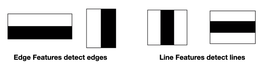
You then extract the features from the images. Figure 1 shows some of the features that are extracted from images containing faces.
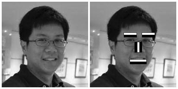
To detect faces from an image, you look for the presence of the various features that are usually found on human faces (see Figure 2), such as the eyebrow, where the region above the eyebrow is lighter than the region below it.
When an image contains a combination of all these features, it is deemed to contain a face.
If you're interested in a visualization of how a face is detected, check out the following videos on YouTube:
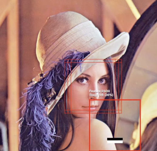
- https://www.youtube.com/watch?v=hPCTwxF0qf4 (see Figure 3)
- https://www.youtube.com/watch?v=F5rysk51txQ
Fortunately, without needing to know how Haar cascades work, OpenCV can perform face detection out of the box using a pre-trained Haar cascade, along with other Haar cascades for recognizing other objects. The list of predefined Haar cascades is available on GitHub at https://github.com/opencv/opencv/tree/master/data/haarcascades.
For face detection, you'll need the haarcascade_frontalface_default.xml file that you can download from the GitHub link in the previous paragraph.
Detecting Faces Using Webcam
Now that you have a basic idea of how face detection works using Haar cascades, let's write a Python program to turn on a webcam and then try to detect the face in it. I'll be using Anaconda.
First, install OpenCV using the following command at the Anaconda Prompt (or Terminal if you are using a Mac):
$ pip install opencv-python
Next, create a file named face_detection.py and populate it with the code shown in Listing 1. Then, download the haarcascade_frontalface_default.xml file and save it into the same directory as the face_detection.py file.
Listing 1: The content of the face_detection.py file
import cv2

# for face detection
face_cascade = \ cv2.CascadeClassifier('haarcascade_frontalface_default.xml')

# resolution of the webcam
screen_width = 1280       # try 640 if code fails
screen_height = 720

# default webcam
stream = cv2.VideoCapture(0)

while(True):
    # capture frame-by-frame
    (grabbed, frame) = stream.read()
    rgb = cv2.cvtColor(frame, cv2.COLOR_BGR2RGB)

    # try to detect faces in the webcam
    faces = face_cascade.detectMultiScale(rgb, scaleFactor=1.3, minNeighbors=5)

    # for each faces found
    for (x, y, w, h) in faces:
        # Draw a rectangle around the face
        color = (0, 255, 255) # in BGR
        stroke = 5
        cv2.rectangle(frame, (x, y), (x + w, y + h), color, stroke)

    # show the frame
    cv2.imshow("Image", frame)
    key = cv2.waitKey(1) & 0xFF
    if key == ord("q"):    # Press q to break out
    break                  # of the loop

# cleanup
stream.release()
cv2.waitKey(1)
cv2.destroyAllWindows()
cv2.waitKey(1)
To run the program, type the following command in Anaconda Prompt:
$ python face_detection.py
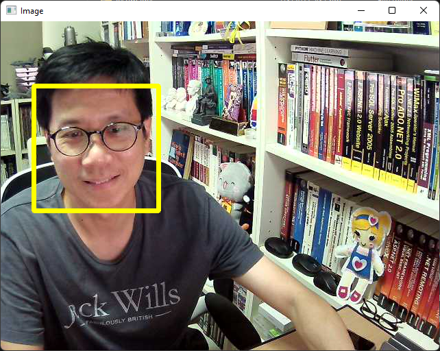
Figure 4 shows that when the program detects a face, it draws a rectangle around it. If it detects multiple faces, multiple rectangles are shown.
Techniques to Recognize Faces
Now that you've learned how to detect faces, you are ready to tackle the bigger challenge of recognizing faces! Face detection is a technique for detecting faces in an image and face recognition is a technique for recognizing faces in an image. Compared to face detection, face recognition is a much more complicated process and is an area of much interest to researchers, who are always looking to improve the accuracy of the recognition.
In this article, I'll discuss two techniques that you can generally use for face recognition:
- Deep learning using convolutional neural networks (CNN)
- Machine learning using support vector machines (SVM)
Deep Learning - Convolutional Neural Network (CNN)
In deep learning, a convolutional neural network (CNN) is a special type of neural network that is designed to process data through multiple layers of arrays. A CNN is well-suited for applications like image recognition and is often used in face recognition software.
In CNN, convolutional layers are the fundamental building blocks that make all the magic happen. In a typical image recognition application, a convolutional layer is made up of several filters to detect the various features of the image. Understanding how this work is best illustrated with an analogy.
Suppose you saw someone walking toward you from a distance. From afar, your eyes will try to detect the edges of the figure, and you try to differentiate that figure from other objects, such as buildings or cars, etc. As the person walks closer toward you, you try to focus on the outline of the person, trying to deduce if the person is male or female, slim or fat, etc. As the person gets nearer, your focus shifts toward other features of that person, such as his facial features, if his is wearing specs, etc. In general, your focus shifts from broad features to specific features.
Likewise, in a CNN, you have several layers containing various filters (or kernels, as they are commonly called) in charge of detecting specific features of the target you're trying to detect. The early layer tries to focus on broad features, while the latter layers try to detect very specific features. In a CNN, the values for the various filters in each convolutional layer is obtained by training on a particular training set. At the end of the training, you have a unique set of filter values that are used for detecting specific features in the dataset. Using this set of filter values, you apply them on new images so that you can make a prediction about what is contained within the image.
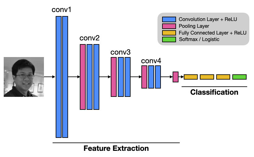
Figure 5 shows a typical CNN network. The first few convolutional layers (conv1 to conv4) detect the various features (from abstract to specific) in an image (such as edges, lines, etc.). The final few layers (the fully connected layers and the final softmax/logistic layer) are used to classify the result (such as that the image contains faces belong to person A, B, or C).
A Pooling layer in CNN is used to reduce the size of the representations and to speed up calculations, as well as to make some of the features it detects a bit more robust.
Using VGGFace for Face Recognition
VGGFace refers to a series of models developed for face recognition. It was developed by the Visual Geometry Group (hence its VGG name) at the University of Oxford. The models were trained on a dataset comprised mainly of celebrities, public figures, actors, and politicians. Their names were extracted from the Internet Movie Data Base (IMDB) celebrity list based on their gender, popularity, pose, illumination, ethnicity, and profession (actors, athletes, politicians). The images of these names were fetched from Google Image Search, and multiple images for each name were downloaded, vetted by humans, and then labelled for training.
There are two versions of VGGFace:
VGGFace: Developed in 2015, trained on 2.6 million images, a total of 2622 people
VGGFace2: Developed in 2017, trained on 3.31 million images, a total of 9131 people
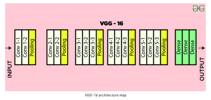
The original VGGFace uses the VGG16 model, which is a convolutional neural network with 16 layers (see Figure 6).
VGGFace2 uses a much larger dataset and two models have been trained using:
- ResNet-50
- SqueezeNet-ResNet-50 (also known as SENet)
ResNet50 is a 50-layer Residual Network with 26M parameters. This residual network is a deep convolutional neural network that was introduced by Microsoft in 2015.
To know more about ResNet-50, go to https://viso.ai/deep-learning/resnet-residual-neural-network/.
SENet is a smaller network developed by researchers at DeepScale, University of California at Berkeley, and Stanford University. The goal of SENet was to create a smaller neural network that can easily fit into computer memory and be easily transmitted over a computer network.
Let's now try out how VGGFace works and see if it can accurately recognize some of the faces that we throw at it. For this, you'll make use of the Keras's implementation of VGGFace located at https://github.com/rcmalli/keras-vggface.
For this example, I'll use Jupyter Notebook. First, you need to install the keras_vggface and keras_applications modules:
!pip install keras_vggface
!pip install keras_applications
The
keras_applicationsmodule provides model definitions and pre-trained weights for a number of popular architectures such as VGG16, ResNet50, Xception, MobileNet, and more.
To use VGGFace (based on the VGG16 CNN model), you can specify the vgg16 argument for the model parameter:
from keras_vggface.vggface import VGGFace

model = VGGFace(model='vgg16')
# same as the following
model = VGGFace() # vgg16 as default
To use VGGFace2 with the ResNet-50 model, you can specify the resnet50 argument:
model = VGGFace(model='resnet50')
To use VGGFace2 with the SENet model, specify the senet50 argument:
model = VGGFace(model='senet50')
For the example here, I'm going to use the SENet model. When you run the above code snippets, the weights for the trained model will be downloaded and stored in the ~/.keras/models/vggface folder. Here's the size (in bytes) of the weights downloaded for each model:
165439116 rcmalli_vggface_tf_resnet50.h5
175688524 rcmalli_vggface_tf_senet50.h5
580070376 rcmalli_vggface_tf_vgg16.h5
As you can observe, the VGG16 weights is the largest at 580 MB and the ResNet50 is smallest at 165 MB.
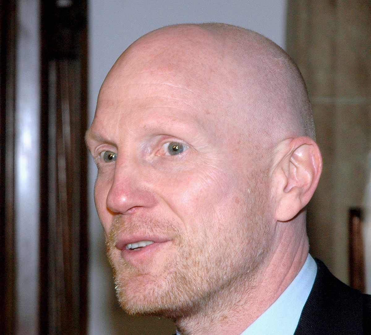
You're now ready to test the model and see if it could recognize a face that it was trained to recognize. The first face that I want to try is Mattias Sammer (see Figure 7), a German former professional football player and coach who last worked as sporting director in Bayern Munich.
Download a copy of his headshot (Matthias_Sammer.jpg) and put it in the same folder as your Jupyter Notebook. The following code snippet will load the image, resize it to 224x224 pixels, convert the image into a NumPy array, and then use the model to make the prediction:
import numpy as np
from keras.preprocessing import image
from keras_vggface.vggface import VGGFace
from keras_vggface import utils

# load the image
img = image.load_img(
    './Matthias_Sammer.jpg',
    target_size=(224, 224))

# prepare the image
x = image.img_to_array(img)
x = np.expand_dims(x, axis=0)
x = utils.preprocess_input(x, version=1)

# perform prediction
preds = model.predict(x)
print('Predicted:', utils.decode_predictions(preds))
The result of the prediction is as follows:
Predicted:
  [[["b' Matthias_Sammer'", 0.9927065],
    ["b' Bj\\xc3\\xb6rn_Ferry'", 0.0011530316],
    ["b' Stone_Cold_Steve_Austin'", 0.00084367086],
    ["b' Florent_Balmont'", 0.00058827153],
    ["b' Tim_Boetsch'", 0.0003584346]]]
From the result, you can see that the probability of the image containing Matthias Sammer's face is 0.9927065 (the highest probability).
Using Transfer Learning to Recognize Custom Faces
The previous section showed how you can use VGGFace2 to recognize some of the pretrained faces. Although this is cool, it isn't very exciting. A more interesting way to use the VGGFace2 is to use it to recognize the faces that you want. For example let's say that you want to use it to build an attendance system to recognize students in a class. To do that, you make use of a technique called transfer learning.
Transfer learning is a machine learning method where a model developed for a task is reused as the starting point for a model on a second task. Transfer learning reduces the amount of time that you need to spend on training.
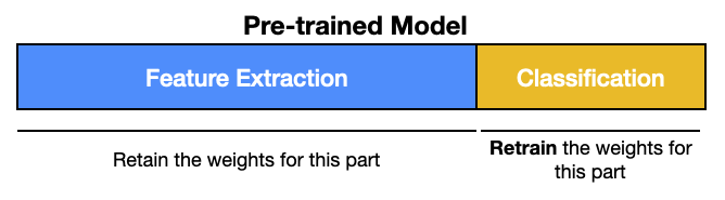
Recall that in general CNN, models for image classification can be divided into two parts:
Feature extraction: the aim of this part is to find the features in the image
Classification: the aim of this part is to use the various features extracted in the previous part and classify the image to the desired classes. For example, if it sees eyes, nose, eyebrows it can tell it's a human face belonging to a specific person
When you do transfer learning, you can retain the feature extraction part of a trained model and only retrain the classifier part (see Figure 8).
Preprocessing the Training Images
To use transfer learning to train a model to recognize faces, you need to first obtain images of the people. For this example, the model will be trained to recognize:
- Barack Obama
- Donald Trump
- Tom Cruise
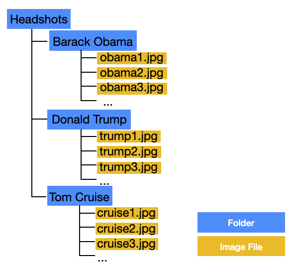
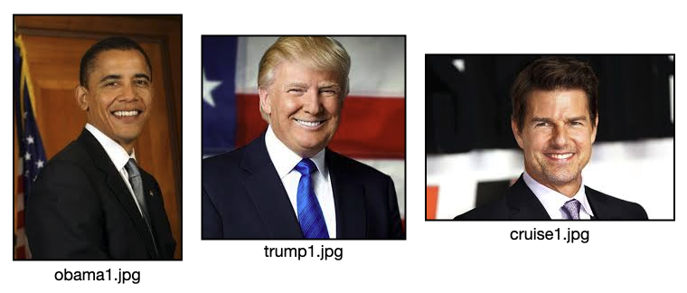
In the folder where you saved your Jupyter Notebook files, create a folder named Headsets and create sub-folders within it using the names of the people you want to train (see Figure 10). Within each sub-folder you have images of the people. Figure 9 shows some of the images in the folders.
The images of each person can be of any size, and you should aim for at least 10 images in each folder.
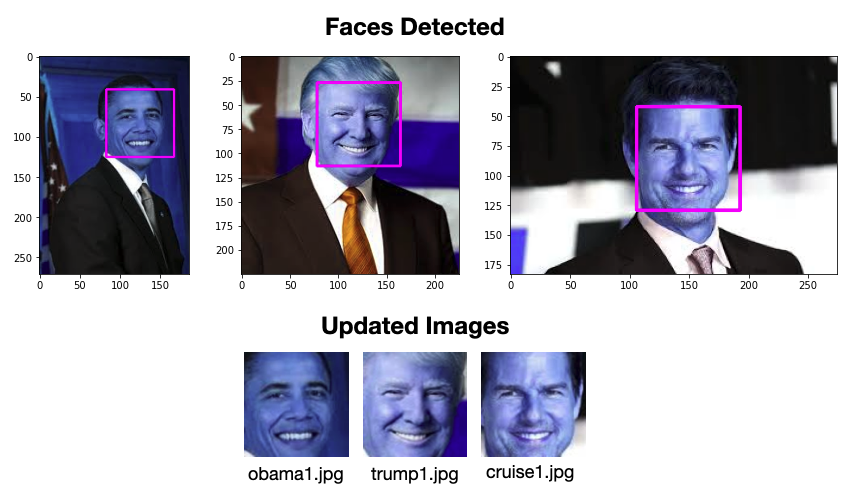
Once the images are prepared and saved in the respective folders, you need to perform some preprocessing on the images before you can use them for training. You need to extract the faces from the images so that only the faces are used for training. The steps are as follows:
- Iterate through all the images in the folders and extract the face in the image using OpenCV's Haar cascade.
- Resize the extracted face to the size required by VGGFace16: 224x224 pixels.
- Replace the original image with the extracted face.
Listing 2 shows the code for preprocessing the images.
Listing 2: Preprocessing the images used for training
import cv2
import os
import pickle
import numpy as np
from PIL import Image

import matplotlib.pyplot as plt

headshots_folder_name = 'Headshots'

# dimension of images
image_width = 224
image_height = 224

# for detecting faces
facecascade = cv2.CascadeClassifier('haarcascade_frontalface_default.xml')

# set the directory containing the images
images_dir = os.path.join(".", headshots_folder_name)

current_id = 0
label_ids = {}

# iterates through all the files in each subdirectories
for root, _, files in os.walk(images_dir):
    for file in files:
        if file.endswith("png") or
        file.endswith("jpg") or
        file.endswith("jpeg"):
        # path of the image
        path = os.path.join(root, file)

        # get the label name (name of the person)
        label = os.path.basename(root).replace(" ", ".").lower()

        # add the label (key) and its number (value)
        if not label in label_ids:
            label_ids[label] = current_id
            current_id += 1

        # load the image
        imgtest = cv2.imread(path, cv2.IMREAD_COLOR)
        image_array = np.array(imgtest, "uint8")

        # get the faces detected in the image
        faces = \ facecascade.detectMultiScale(imgtest,
            scaleFactor=1.1, minNeighbors=5)

        # if not exactly 1 face is detected, skip this photo
        if len(faces) != 1:
            print(f'---Photo skipped---\n')
        # remove the original image
        os.remove(path)
        continue

        # save the detected face(s) and associate
        # them with the label
        for (x_, y_, w, h) in faces:

            # draw the face detected
            face_detect = cv2.rectangle(imgtest,
                    (x_, y_),
                    (x_+w, y_+h),
                    (255, 0, 255), 2)
            plt.imshow(face_detect)
            plt.show()

            # resize the detected face to 224x224
            size = (image_width, image_height)

            # detected face region
            roi = image_array[y_: y_ + h, x_: x_ + w]

            # resize the detected head to target size
            resized_image = cv2.resize(roi, size)
            image_array = np.array(resized_image, "uint8")

            # remove the original image
            os.remove(path)

            # replace the image with only the face
            im = Image.fromarray(image_array)
            im.save(path)
Figure 11 shows the face detected in each image and the updated images. It's possible that in some images there will be multiple faces detected. In the event that there is no face or when there are multiple faces detected, the image is discarded.
Importing the Libraries
You're now ready to train a model using the faces that you extracted in the previous section. First, let's import the various modules that you need:
import os
import pandas as pd
import numpy as np
import tensorflow.keras as keras
import matplotlib.pyplot as plt

from tensorflow.keras.layers
    import Dense, GlobalAveragePooling2D

from tensorflow.keras.preprocessing import image
from tensorflow.keras.applications.mobilenet
    import preprocess_input

from tensorflow.keras.preprocessing.image
   import ImageDataGenerator

from tensorflow.keras.models import Model

from tensorflow.keras.optimizers import Adam
Augmenting the Training Images
You use the ImageDataGenerator class to augment the images that you have for training. The ImageDataGenerator class applies different transformations to your images (so that one single image can be transformed into different images, which is useful when you have a very limited number of images for training) when you are training the model.
The
ImageDataGeneratorclass performs image augmentation, a very useful technique when you don't have enough training data to train your model.
train_datagen = ImageDataGenerator(
    preprocessing_function=preprocess_input)

train_generator = \
    train_datagen.flow_from_directory(
'./Headshots',
target_size=(224,224),
color_mode='rgb',
batch_size=32,
class_mode='categorical',
shuffle=True)
The flow_from_directory() function from the ImageDataGenerator instance generates a tf.data.Dataset from image files in the specified directory. Using the result, you can find out how many classes of images you have:
train_generator.class_indices.values()
# dict_values([0, 1, 2])
NO_CLASSES = \len(train_generator.class_indices.values())
Building the Model
Next, you're ready to build the model. First, load the VGGFace16 model:
from keras_vggface.vggface import VGGFace

base_model = VGGFace(include_top=True,
    model='vgg16',
    input_shape=(224, 224, 3))
base_model.summary()

print(len(base_model.layers))
# 26 layers in the original VGG-Face
The model is shown in Listing 3. As you can see, there are 26 layers in the VGGFace16 model altogether. These seven layers represent the three fully connected output layers used to recognize faces.
base_model = VGGFace(include_top=False,
model='vgg16',
input_shape=(224, 224, 3))
base_model.summary()
print(len(base_model.layers))
# 19 layers after excluding the last few layers
Listing 3: The various layers in VGGFace16
Model: "vggface_vgg16"
_________________________________________________________________
Layer (type)                 Output Shape              Param #
=================================================================
input_1 (InputLayer)         [(None, 224, 224, 3)]     0
_________________________________________________________________
conv1_1 (Conv2D)             (None, 224, 224, 64)      1792
_________________________________________________________________
conv1_2 (Conv2D)             (None, 224, 224, 64)      36928
_________________________________________________________________
pool1 (MaxPooling2D)         (None, 112, 112, 64)      0
_________________________________________________________________
conv2_1 (Conv2D)             (None, 112, 112, 128)     73856
_________________________________________________________________
conv2_2 (Conv2D)             (None, 112, 112, 128)     147584
_________________________________________________________________
pool2 (MaxPooling2D)         (None, 56, 56, 128)       0
_________________________________________________________________
conv3_1 (Conv2D)             (None, 56, 56, 256)       295168
_________________________________________________________________
conv3_2 (Conv2D)             (None, 56, 56, 256)       590080
_________________________________________________________________
conv3_3 (Conv2D)             (None, 56, 56, 256)       590080
_________________________________________________________________
pool3 (MaxPooling2D)         (None, 28, 28, 256)       0
_________________________________________________________________
conv4_1 (Conv2D)             (None, 28, 28, 512)       1180160
_________________________________________________________________
conv4_2 (Conv2D)             (None, 28, 28, 512)       2359808
_________________________________________________________________
conv4_3 (Conv2D)             (None, 28, 28, 512)       2359808
_________________________________________________________________
pool4 (MaxPooling2D)         (None, 14, 14, 512)       0
_________________________________________________________________
conv5_1 (Conv2D)             (None, 14, 14, 512)       2359808
_________________________________________________________________
conv5_2 (Conv2D)             (None, 14, 14, 512)       2359808
_________________________________________________________________
conv5_3 (Conv2D)             (None, 14, 14, 512)       2359808
_________________________________________________________________
pool5 (MaxPooling2D)         (None, 7, 7, 512)         0
_________________________________________________________________
flatten (Flatten)            (None, 25088)             0
_________________________________________________________________
fc6 (Dense)                  (None, 4096)              102764544
_________________________________________________________________
fc6/relu (Activation)        (None, 4096)              0
_________________________________________________________________
fc7 (Dense)                  (None, 4096)              16781312
_________________________________________________________________
fc7/relu (Activation)        (None, 4096)              0
_________________________________________________________________
fc8 (Dense)                  (None, 2622)              10742334
_________________________________________________________________
fc8/softmax (Activation)     (None, 2622)              0
=================================================================
Total params: 145,002,878
Trainable params: 145,002,878
Non-trainable params: 0
_________________________________________________________________
26
If you run the above code snippet, you'll see that the output now only has 19 layers. The last seven layers (representing the three fully connected output layers) are no longer loaded.
Let's now add the custom layers so that the model can recognize the faces in your own training images:
x = base_model.output
x = GlobalAveragePooling2D()(x)

x = Dense(1024, activation='relu')(x)
x = Dense(1024, activation='relu')(x)
x = Dense(512, activation='relu')(x)

# final layer with softmax activation
preds = Dense(NO_CLASSES, activation='softmax')(x)
Listing 4 shows the additional layers that you've just added:
Listing 4: The VGGFace16 now includes the additional layers that you have added to it
Model: "model"
_________________________________________________________________
Layer (type)                 Output Shape              Param #
=================================================================

...

conv5_3 (Conv2D)             (None, 14, 14, 512)       2359808
_________________________________________________________________
pool5 (MaxPooling2D)         (None, 7, 7, 512)         0
_________________________________________________________________
global_average_pooling2d     (Gl (None, 512)           0
_________________________________________________________________
dense (Dense)                (None, 1024)              525312
_________________________________________________________________
dense_1 (Dense)              (None, 1024)              1049600
_________________________________________________________________
dense_2 (Dense)              (None, 512)               524800
_________________________________________________________________
dense_3 (Dense)              (None, 3)                 1539
=================================================================
Total params: 16,815,939
Trainable params: 16,815,939
Non-trainable params: 0
_________________________________________________________________
Finally, set the first 19 layers to be non-trainable and the rest of the layers to be trainable:
# create a new model with the base model's original input and the
# new model's output
model = Model(inputs = base_model.input, outputs = preds)
model.summary()

# don't train the first 19 layers - 0..18
for layer in model.layers[:19]:
    layer.trainable = False

# train the rest of the layers - 19 onwards
for layer in model.layers[19:]:
    layer.trainable = True
Because the first 19 layers were already trained by the VGGFace16 model, you only need to train the new layers that you've added to the model. Essentially, the new layers that you've added will be trained to recognize your own images.
Compiling and Training the Model
You can now compile the model using the Adam optimizer and the categorical Entropy loss function:
model.compile(optimizer='Adam',
    loss='categorical_crossentropy',
    metrics=['accuracy'])
Finally, train the model using the following arguments:
model.fit(train_generator,
  batch_size = 1,
  verbose = 1,
  epochs = 20)
Saving the Model
Once the model is trained, it's important to save it to disk first. If not, you must train the model again every time you want to recognize a face:
# creates a HDF5 file
model.save(
    'transfer_learning_trained' +
    '_face_cnn_model.h5')
To verify that the model is saved correctly, delete it from memory and load it from disk again:
from tensorflow.keras.models
    import load_model

# deletes the existing model
del model

# returns a compiled model identical to the previous one
model = load_model(
    'transfer_learning_trained' +
    '_face_cnn_model.h5')
Saving the Training Labels
Using the ImageDataGenerator instance, you can generate a mapping of the index corresponding to each person's name:
import pickle

class_dictionary = \train_generator.class_indices
class_dictionary = {
    value:key for key, value in class_dictionary.items()
}
print(class_dictionary)
The above code prints out the following:
{
    0: 'Barack Obama',
    1: 'Donald Trump',
    2: 'Tom Cruise'
}
This dictionary is needed so that later on when you perform a prediction, you can use the result returned by the model (which is an integer and not the person's name) to get the person's name.
Save the dictionary object using Pickle:
# save the class dictionary to pickle
face_label_filename = 'face-labels.pickle'
with open(face_label_filename, 'wb') as f: pickle.dump(class_dictionary, f)
Testing the Trained Model
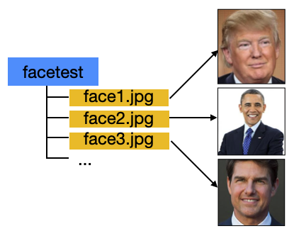
In the folder where you saved your Jupyter Notebook files, create a folder named facetest and add samples of images containing faces of the people you want to recognize. Figure 12 shows some of the images in the folders.
Import the modules and load the labels for the various faces:
import cv2
import os
import pickle
import numpy as np
import pickle

from PIL import Image
import matplotlib.pyplot as plt
from keras.preprocessing import image
from keras_vggface import utils

# dimension of images
image_width = 224
image_height = 224

# load the training labels
face_label_filename = 'face-labels.pickle'
with open(face_label_filename, "rb") as \
    f: class_dictionary = pickle.load(f)

class_list = [value for _, value in class_dictionary.items()]
print(class_list)
The loaded face label is a dictionary containing the mapping of integer values to the names of the people that you have trained. The above code snippet converted that dictionary into a list that looks like this:
['Barack Obama', 'Donald Trump', 'Tom Cruise']
Later on, after the prediction, you'll make use of this list to obtain the name of the predicted face.
Listing 5 shows how to iterate through all the images in the facetest folder and send the image to the model for prediction.
Listing 5: Predicting the faces
# for detecting faces
facecascade = \ cv2.CascadeClassifier(
'haarcascade_frontalface_default.xml')
for i in range(1,30): test_image_filename = f'./facetest/face{i}.jpg'
# load the image
imgtest = cv2.imread(test_image_filename, cv2.IMREAD_COLOR)
image_array = np.array(imgtest, "uint8")
# get the faces detected in the image
faces = facecascade.detectMultiScale(imgtest,
scaleFactor=1.1, minNeighbors=5)
# if not exactly 1 face is detected, skip this photo
if len(faces) != 1:
print(f'---We need exactly 1 face;
photo skipped---')
print()
continue
for (x_, y_, w, h) in faces:
# draw the face detected
face_detect = cv2.rectangle(
imgtest, (x_, y_), (x_+w, y_+h), (255, 0, 255), 2)
plt.imshow(face_detect)
plt.show()
# resize the detected face to 224x224
size = (image_width, image_height)
roi = image_array[y_: y_ + h, x_: x_ + w]
resized_image = cv2.resize(roi, size)
# prepare the image for prediction
x = image.img_to_array(resized_image)
x = np.expand_dims(x, axis=0)
x = utils.preprocess_input(x, version=1)
# making prediction
predicted_prob = model.predict(x)
print(predicted_prob)
print(predicted_prob[0].argmax())
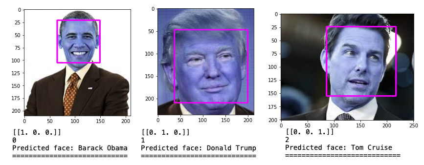
print("Predicted face: " + class_list[predicted_prob[0].argmax()])
print("============================\n")
Figure 13 shows some of the results.
Face Recognition Using Webcam
With the model trained to recognize faces belonging to Obama, Trump, and Cruise, it would be fun to be able to recognize their faces using the webcam. Listing 6 shows how you can use the webcam to perform the prediction in real-time.
Listing 6: Recognizing the face in real-time
from PIL import Image
import numpy as np
import cv2
import pickle
from tensorflow.keras.models import load_model

# for face detection
face_cascade = \ cv2.CascadeClassifier(
    'haarcascade_frontalface_default.xml')

# resolution of the webcam
screen_width = 1280       # try 640 if code fails
screen_height = 720

# size of the image to predict
image_width = 224
image_height = 224

# load the trained model
model = load_model('transfer_learning_trained_face_cnn_model.h5')

# the labels for the trained model
with open("face-labels.pickle", 'rb') as f:
    og_labels = pickle.load(f)
    labels = {key:value for key,value in og_labels.items()}
    print(labels)

# default webcam
stream = cv2.VideoCapture(0)

while(True):
    # Capture frame-by-frame
    (grabbed, frame) = stream.read()
    rgb = cv2.cvtColor(frame, cv2.COLOR_BGR2RGB)

    # try to detect faces in the webcam
    faces = face_cascade.detectMultiScale(
        rgb, scaleFactor=1.3, minNeighbors=5)

    # for each faces found
    for (x, y, w, h) in faces: roi_rgb = rgb[y:y+h, x:x+w]

        # Draw a rectangle around the face
        color = (255, 0, 0) # in BGR
        stroke = 2
        cv2.rectangle(frame, (x, y), (x + w, y + h), color, stroke)

        # resize the image
        size = (image_width, image_height)
        resized_image = cv2.resize(roi_rgb, size)
        image_array = np.array(resized_image, "uint8")
        img = image_array.reshape(1,image_width,image_height,3)
        img = img.astype('float32')
        img /= 255

        # predict the image
        predicted_prob = model.predict(img)

        # Display the label
        font = cv2.FONT_HERSHEY_SIMPLEX
        name = labels[predicted_prob[0].argmax()]
        color = (255, 0, 255)
        stroke = 2
        cv2.putText(frame, f'({name})', (x,y-8),
            font, 1, color, stroke, cv2.LINE_AA)

        # Show the frame
        cv2.imshow("Image", frame)
        key = cv2.waitKey(1) & 0xFF
        if key == ord("q"):    # Press q to break out of the loop
            break

# Cleanup
stream.release()
cv2.waitKey(1)
cv2.destroyAllWindows()
cv2.waitKey(1)
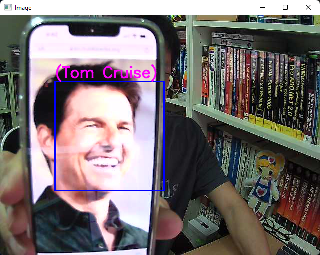
Figure 14 shows the application recognizing the face of Tom Cruise.
Support Vector Machines (SVM)
Another way to perform face recognition is to use support vector machines (SVM). SVMs are a set of supervised learning methods that can be used for classifications. SVM finds the boundary that separates classes by as wide a margin as possible. The main idea behind SVM is to draw a line between two or more classes in the best possible manner (see Figure 15).
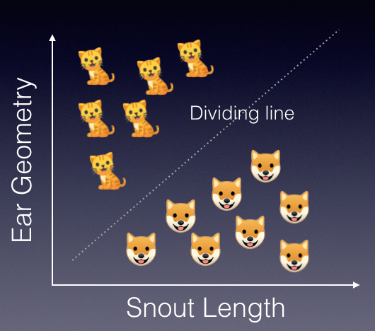
Once the line is drawn to separate the classes, you can then use it to predict future data. For example, given the snout length and ear geometry of a new unknown animal, you can now use the dividing line as a classifier to predict whether the animal is a dog or a cat.
For the following sections, let's use SVM to perform face recognition based on the set of test images that you used in the previous section.
Importing the Packages
First, install the scikit-image module:
!pip install scikit-image
Then, import all the modules that you need:
import os
import pandas as pd
import numpy as np

from sklearn import svm
from sklearn.model_selection import GridSearchCV
from sklearn.model_selection import train_test_split

from sklearn.metrics import classification_report,
    accuracy_score, confusion_matrix

import matplotlib.pyplot as plt
from skimage.transform import resize
from skimage.io import imread

import pickle
Loading the Training Images
Because all the images in the Headshots folder have been preprocessed (with the faces extracted), you can go ahead and load the faces and save them into a Pandas DataFrame (see Listing 7).
Listing 7: Loading all the face images into a Pandas DataFrame
import os
import imageio
import matplotlib.pyplot as plt
new_image_size = (150,150,3)
# set the directory containing the images
images_dir = './Headshots'
current_id = 0
# for storing the foldername: label,
label_ids = {}
# for storing the images data and labels
images = []
labels = []
for root, _, files in os.walk(images_dir):
for file in files:
if file.endswith(('png','jpg','jpeg')):
# path of the image
path = os.path.join(root, file)
# get the label name
label = os.path.basename(root).replace(
" ", ".").lower()
# add the label (key) and its number (value)
if not label in label_ids:
label_ids[label] = current_id
current_id += 1
# save the target value
labels.append(current_id-1)
# load the image, resize and flatten it
image = imread(path)
image = resize(image, new_image_size)
images.append(image.flatten())
# show the image
plt.imshow(image, cmap=plt.cm.gray_r,
interpolation='nearest')
plt.show()
print(label_ids)
# save the labels for each fruit as a list
categories = list(label_ids.keys())
pickle.dump(categories, open("faces_labels.pk", "wb" ))
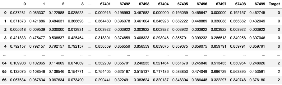
df = pd.DataFrame(np.array(images))
df['Target'] = np.array(labels)
df
The dataframe will look like Figure 16. Each image is loaded and then resized to a dimension of 150x150, with a color depth of three channels (RGB). Each image is flattened and then saved - each pixel is saved as a column in the dataframe (hence there are 15x150x3 columns in the dataframe representing each image). The last column in the dataframe specifies who the face belongs to.
Splitting the Dataset for Training and Testing
Once the images are loaded into the dataframe, you need to split the dataframe into a training and testing set:
x = df.iloc[:,:-1]
y = df.iloc[:,-1]

x_train, x_test, y_train, y_test = \
    train_test_split(x, y,
        test_size = 0.10,    # 10% for test
        random_state=77,
        stratify = y)
Fine Tuning the Best Model Using GridSearchCV
Before you go ahead and start training your model using SVM, you need to fine-tune the hyperparameters of your model so that your model works well with the dataset you have. To do so, you can use the GridSearchCV function in the sklearn module.
GridSearchCV is a function that is in sklearn's model_selection package. It allows you to specify the different values for each hyperparameter and try out all the possible combinations when fitting your model. It does the training and testing using cross validation of your dataset, hence the acronym CV in GridSearchCV. The end result of GridSearchCV is a set of hyperparameters that best fit your data according to the scoring metric that you want your model to optimize on.
For this example, specify the various values for the C, gamma, and kernel hyperparameters:
# trying out the various parameters
param_grid = {
    'C': [0.1, 1, 10, 100],
    'gamma' : [0.0001, 0.001, 0.1,1],
    'kernel' : ['rbf', 'poly']
}

svc = svm.SVC(probability=True)
print("Starting training, please wait ...")

# exhaustive search over specified hyper parameter
# values for an estimator
model = GridSearchCV(svc,param_grid)
model.fit(x_train, y_train)

# print the parameters for the best performing model
print(model.best_params_)
After a while, you should see something like the following (based on my dataset of images):
{'C': 10, 'gamma': 0.0001, 'kernel': 'rbf'}
At this moment, you have also trained a model using the above parameters.
Finding the Accuracy
With the model trained, you want to use the test set to see how your model performs:
y_pred = model.predict(x_test)
print(f"The model is {accuracy_score(y_pred,y_test) * 100}% accurate")
For my dataset, I get the following result:
The model is 85.71428571428571% accurate
I will now save the trained model onto disk:
pickle.dump(model, open('faces_model.pickle','wb'))
Making Predictions
Finally, let's use the set of test faces to see how well the model performs (see Listing 8).
Listing 8: Testing the model
import cv2
import pickle
# loading the model and label
model = pickle.load(open('faces_model.pickle','rb'))
categories = pickle.load(open('faces_labels.pk', 'rb'))
# for detecting faces
facecascade = cv2.CascadeClassifier(
'haarcascade_frontalface_default.xml')
for i in range(1,40):
test_image_filename = f'./facetest/face{i}.jpg'
# load the image
imgtest = cv2.imread(test_image_filename, cv2.IMREAD_COLOR)
image_array = np.array(imgtest, "uint8")
# get the faces detected in the image
faces = facecascade.detectMultiScale(imgtest,
scaleFactor = 1.1, minNeighbors = 5)
# if not exactly 1 face is detected,
# skip this photo
if len(faces) != 1:
print(f'---We need exactly 1 face; photo skipped---\n')
continue
for (x_, y_, w, h) in faces:
# draw the face detected
face_detect = cv2.rectangle(
imgtest, (x_, y_), (x_+w, y_+h),
(255, 0, 255), 2)
plt.imshow(face_detect)
plt.show()
# resize and flatten the face data
roi = image_array[y_: y_ + h, x_: x_ + w]
img_resize = resize(roi, new_image_size)
flattened_image = [img_resize.flatten()]
# predict the probability
probability = \ model.predict_proba(flattened_image)
for i, val in enumerate(categories):
print(f'{val}={probability[0][i] * 100}%')
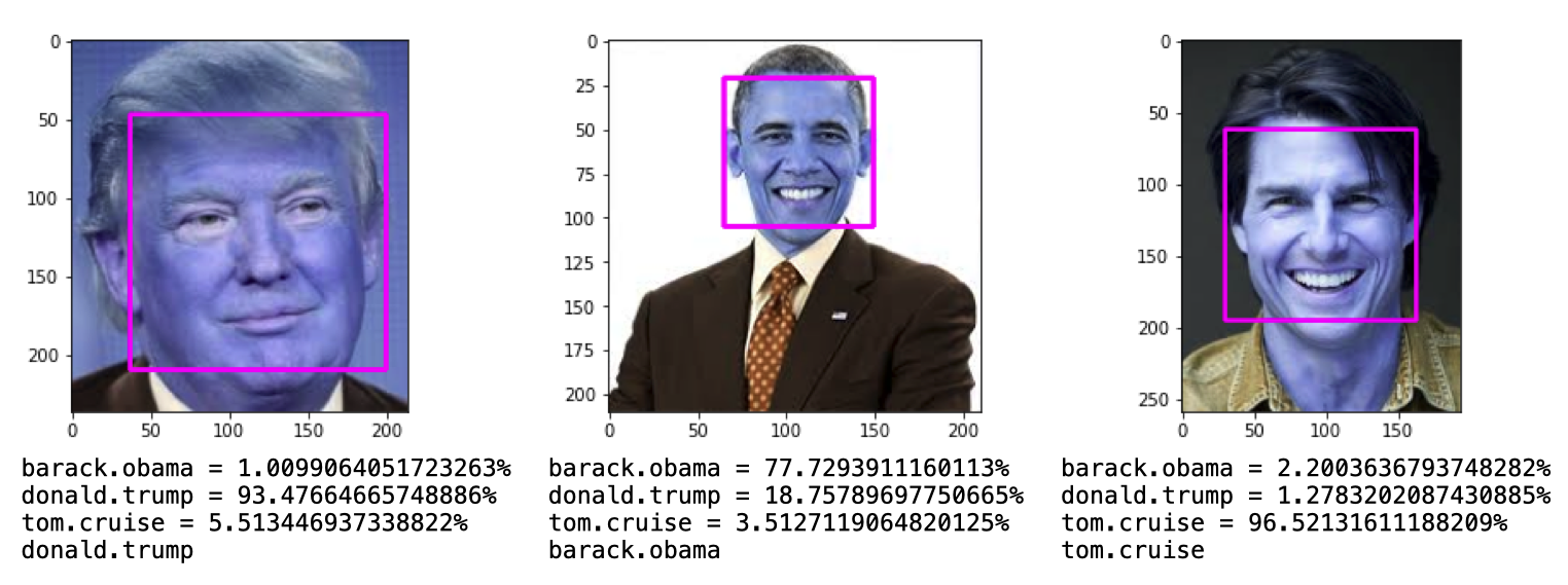
print(f"{categories[model.predict(flattened_image)[0]]}")
Figure 17 shows some of the positive results.
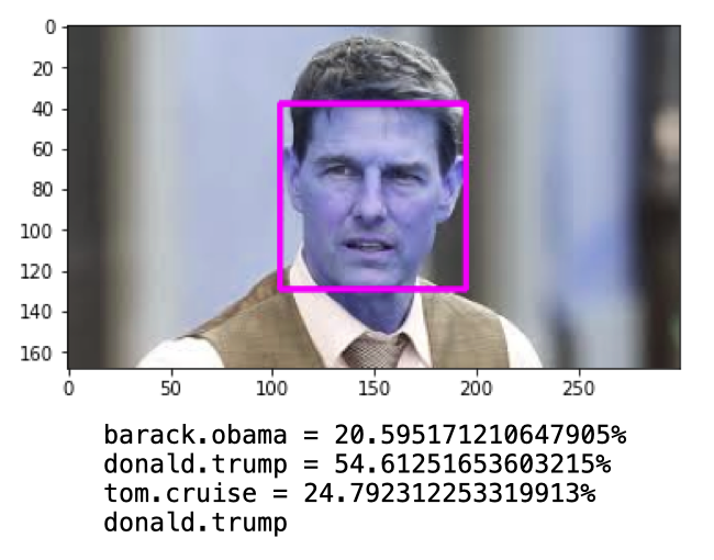
However, there are also some misses (see Figure 18).
Summary
I've attempted to cover a few huge topics in the span of a single article. One topic that I briefly touched on was convolutional neural network (CNN), which, by itself is a topic that requires an entire book to cover in detail. Nevertheless, I hope you now have a good idea of how to perform face recognition using the various libraries covered in this article. There are some other techniques and tools that you can also use, but I will leave it for another day. Have fun!